Euler–Maruyama Method on:
[Wikipedia]
[Google]
[Amazon]
In
 An area that has benefited significantly from SDE is biology or more precisely
# -*- coding: utf-8 -*-
import numpy as np
import matplotlib.pyplot as plt
class Model:
"""
Stochastic model constants.
"""
THETA = 0.7
MU = 1.5
SIGMA = 0.06
def mu(y: float, _t: float) -> float:
"""
Implement the Ornstein–Uhlenbeck mu.
"""
return Model.THETA * (Model.MU - y)
def sigma(_y: float, _t: float) -> float:
"""
Implement the Ornstein–Uhlenbeck sigma.
"""
return Model.SIGMA
def dW(delta_t: float) -> float:
"""
Sample a random number at each call.
"""
return np.random.normal(loc=0.0, scale=np.sqrt(delta_t))
def run_simulation():
"""
Return the result of one full simulation.
"""
T_INIT = 3
T_END = 7
N = 1000 # Compute at 1000 grid points
DT = float(T_END - T_INIT) / N
TS = np.arange(T_INIT, T_END + DT, DT)
assert TS.size N + 1
Y_INIT = 0
ys = np.zeros(TS.size)
ys = Y_INIT
for i in range(1, TS.size):
t = T_INIT + (i - 1) * DT
y = ys - 1 ys = y + mu(y, t) * DT + sigma(y, t) * dW(DT)
return TS, ys
def plot_simulations(num_sims: int):
"""
Plot several simulations in one image.
"""
for _ in range(num_sims):
plt.plot(*run_simulation())
plt.xlabel("time")
plt.ylabel("y")
plt.show()
if __name__"__main__":
NUM_SIMS = 5
plot_simulations(NUM_SIMS)
 The following is simply the translation of the above code into the MATLAB (R2019b) programming language:
%% Initialization and Utility
close all;
clear all;
numSims = 5; % display five runs
tBounds = 7 % The bounds of t
N = 1000; % Compute at 1000 grid points
dt = (tBounds(2) - tBounds(1)) / N ;
y_init = 0; % Initial y condition
% Initialize the probability distribution for our
% random variable with mean 0 and stdev of sqrt(dt)
pd = makedist('Normal',0,sqrt(dt));
c = .7, 1.5, 0.06 % Theta, Mu, and Sigma, respectively
ts = linspace(tBounds(1), tBounds(2), N); % From t0-->t1 with N points
ys = zeros(1,N); % 1xN Matrix of zeros
ys(1) = y_init;
%% Computing the Process
for j = 1:numSims
for i = 2:numel(ts)
t = tBounds(1) + (i-1) .* dt;
y = ys(i-1);
mu = c(1) .* (c(2) - y);
sigma = c(3);
dW = random(pd);
ys(i) = y + mu .* dt + sigma .* dW;
end
figure;
hold on;
plot(ts, ys, 'o')
end
Itô calculus
Itô calculus, named after Kiyosi Itô, extends the methods of calculus to stochastic processes such as Brownian motion (see Wiener process). It has important applications in mathematical finance and stochastic differential equations.
The centra ...
, the Euler–Maruyama method (also called the Euler method) is a method for the approximate numerical solution
Numerical analysis is the study of algorithms that use numerical approximation (as opposed to symbolic manipulations) for the problems of mathematical analysis (as distinguished from discrete mathematics). It is the study of numerical methods th ...
of a stochastic differential equation
A stochastic differential equation (SDE) is a differential equation in which one or more of the terms is a stochastic process, resulting in a solution which is also a stochastic process. SDEs are used to model various phenomena such as stock pr ...
(SDE). It is an extension of the Euler method
In mathematics and computational science, the Euler method (also called forward Euler method) is a first-order numerical procedure for solving ordinary differential equations (ODEs) with a given initial value. It is the most basic explicit met ...
for ordinary differential equation
In mathematics, an ordinary differential equation (ODE) is a differential equation whose unknown(s) consists of one (or more) function(s) of one variable and involves the derivatives of those functions. The term ''ordinary'' is used in contrast w ...
s to stochastic differential equations. It is named after Leonhard Euler
Leonhard Euler ( , ; 15 April 170718 September 1783) was a Swiss mathematician, physicist, astronomer, geographer, logician and engineer who founded the studies of graph theory and topology and made pioneering and influential discoveries in ma ...
and Gisiro Maruyama. Unfortunately, the same generalization cannot be done for any arbitrary deterministic method.
Consider the stochastic differential equation (see Itô calculus
Itô calculus, named after Kiyosi Itô, extends the methods of calculus to stochastic processes such as Brownian motion (see Wiener process). It has important applications in mathematical finance and stochastic differential equations.
The centra ...
)
:
with initial condition
In mathematics and particularly in dynamic systems, an initial condition, in some contexts called a seed value, is a value of an evolving variable at some point in time designated as the initial time (typically denoted ''t'' = 0). For ...
''X''0 = ''x''0, where ''W''''t'' stands for the Wiener process
In mathematics, the Wiener process is a real-valued continuous-time stochastic process named in honor of American mathematician Norbert Wiener for his investigations on the mathematical properties of the one-dimensional Brownian motion. It is o ...
, and suppose that we wish to solve this SDE on some interval of time , ''T'' Then the Euler–Maruyama approximation to the true solution ''X'' is the Markov chain
A Markov chain or Markov process is a stochastic model describing a sequence of possible events in which the probability of each event depends only on the state attained in the previous event. Informally, this may be thought of as, "What happe ...
''Y'' defined as follows:
* partition the interval , ''T''into ''N'' equal subintervals of width :
::
* set ''Y''0 = ''x''0
* recursively define ''Y''''n'' for 0 ≤ ''n'' ≤ ''N-1'' by
::
:where
::
The random variable
A random variable (also called random quantity, aleatory variable, or stochastic variable) is a mathematical formalization of a quantity or object which depends on random events. It is a mapping or a function from possible outcomes (e.g., the po ...
s Δ''W''''n'' are independent and identically distributed
In probability theory and statistics, a collection of random variables is independent and identically distributed if each random variable has the same probability distribution as the others and all are mutually independent. This property is usua ...
normal random variables with expected value
In probability theory, the expected value (also called expectation, expectancy, mathematical expectation, mean, average, or first moment) is a generalization of the weighted average. Informally, the expected value is the arithmetic mean of a l ...
zero and variance
In probability theory and statistics, variance is the expectation of the squared deviation of a random variable from its population mean or sample mean. Variance is a measure of dispersion, meaning it is a measure of how far a set of numbers ...
.
Example
Numerical simulation
 An area that has benefited significantly from SDE is biology or more precisely
 mathematical biology
Mathematical and theoretical biology, or biomathematics, is a branch of biology which employs theoretical analysis, mathematical models and abstractions of the living organisms to investigate the principles that govern the structure, development a ...
. Here the number of publications on the use of stochastic model grew, as most of the models are nonlinear, demanding numerical schemes.
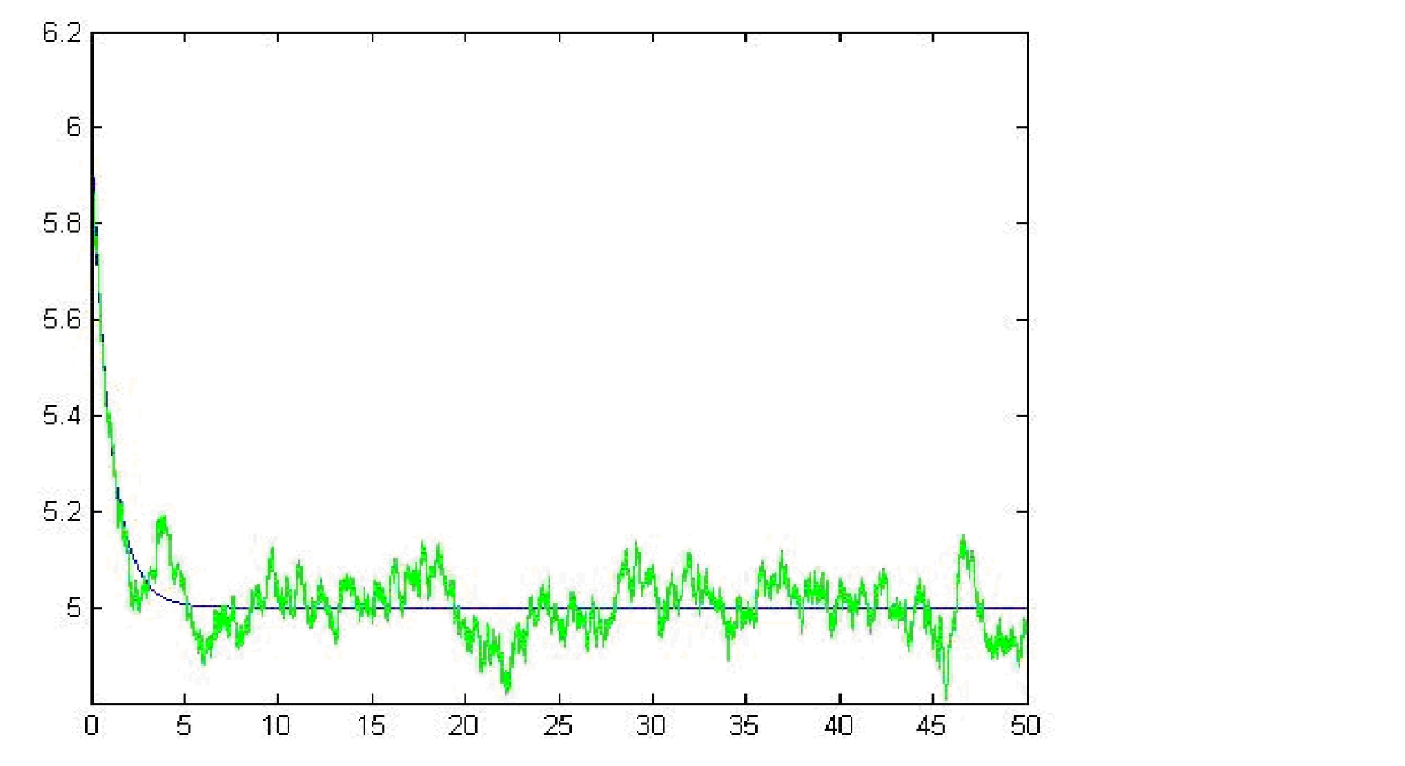
The graphic depicts a stochastic differential equation being solved using the Euler Scheme. The deterministic counterpart is shown as well.
Computer implementation
The followingPython
Python may refer to:
Snakes
* Pythonidae, a family of nonvenomous snakes found in Africa, Asia, and Australia
** ''Python'' (genus), a genus of Pythonidae found in Africa and Asia
* Python (mythology), a mythical serpent
Computing
* Python (pro ...
code implements the Euler–Maruyama method and uses it to solve the Ornstein–Uhlenbeck process
In mathematics, the Ornstein–Uhlenbeck process is a stochastic process with applications in financial mathematics and the physical sciences. Its original application in physics was as a model for the velocity of a massive Brownian particle ...
defined by
:
:
The random numbers for are generated using the NumPy mathematics package.
 The following is simply the translation of the above code into the MATLAB (R2019b) programming language:
See also
*Milstein method
In mathematics, the Milstein method is a technique for the approximate numerical solution of a stochastic differential equation. It is named after Grigori N. Milstein who first published it in 1974.
Description
Consider the autonomous Itō stoch ...
* Runge–Kutta method (SDE)
* Leimkuhler–Matthews method
References
{{DEFAULTSORT:Euler-Maruyama method Numerical differential equations Stochastic differential equations Leonhard Euler Articles with example Python (programming language) code Articles with example MATLAB/Octave code